Fundamentals of Structural-Acoustic Analysis in Abaqus

Introduction

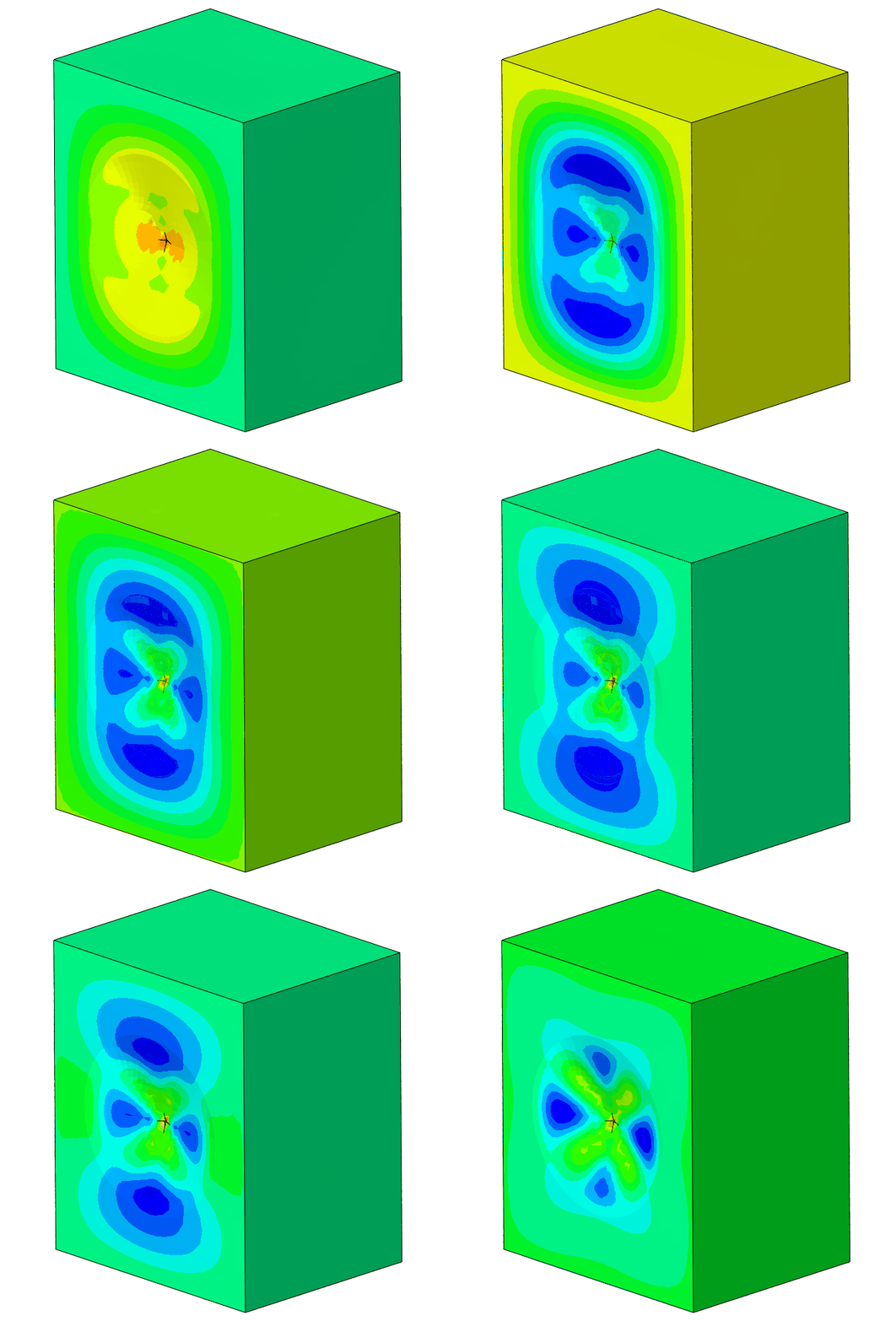
Abaqus features specialized finite elements designed to model acoustic media. When combined with dynamic analysis procedures, these elements enable the simulation of low-amplitude wave phenomena in fluids—such as air and water—as well as higher-amplitude shock wave analyses involving fluid-structure interaction.

Acoustic analyses allow for the simulation of the acoustic medium in isolation (e.g., modal analysis of a fluid-filled cavity) or coupled structural-acoustic systems (e.g., vehicle noise levels or sound propagation within a coupled system). This analysis technique is suitable for both internal problems, where a structure encloses one or more fluid-filled spaces, and external problems, where a structure is immersed in a fluid medium extending to infinity. The fundamental assumption is that wave propagation occurs solely through compression and expansion of the medium, without shear effects; the model assumes small-amplitude vibrations in a medium that lacks shear stiffness. An acoustic medium can even be a solid material (such as rubber or soil), provided that shear effects are considered negligible.

Shock wave analyses, on the other hand, allow for modeling the impact of explosions on structures and can utilize the CONWEP air-blast loading model in Abaqus/Explicit. Incident wave loading models are also available for acoustic analyses, including the UNDEX model for underwater explosions; however, this article does not focus on these types of loading. Analyses involving acoustic elements assume small deformations (specifically, or predominantly, volumetric in nature). Acoustic pressure is linearly proportional to the volumetric deformation of the medium that induces it. This assumption can hold true even with large changes in pressure and density—such as in the case of shock waves in water—whereas small changes are typically assumed. However, powerful explosions in air and close-range underwater explosions do not satisfy this assumption. The medium possesses inertia, which resists accelerations caused by the medium's volume changes. Waves may also be attenuated by viscosity. Certain nonlinear acoustic models, such as time-domain volumetric cavitation, can also be analyzed.

Unlike hydrodynamics, acoustics assumes fluid compressibility (finite wave speed) and that wave speed is independent of frequency. These theories align at low frequencies and over long time scales.

Supported analysis procedures

Both time-domain and frequency-domain procedures are supported: *STEADY STATE DYNAMICS (MODE BASED/DIRECT/SUBSPACE PROJECTION), *FREQUENCY, *COMPLEX FREQUENCY, *DYNAMIC (implicit/explicit), *MODAL DYNAMIC, and *DYNAMIC TEMPERATURE-DISPLACEMENT (explicit). The direct SSD procedure is generally recommended due to the absence of approximations across ranges (albeit at the cost of longer computation times). The explicit dynamics procedure is suitable for short-duration shock events and can account for acoustic material nonlinearity in the form of cavitation. Conversely, the implicit dynamics procedure is primarily used for analyzing long-duration processes dominated by low-frequency response; in this case, the acoustic response is linear. Acoustic elements with linear interpolation perform best.

In static analyses, all acoustic effects are ignored. However, such an analysis may precede a dynamic procedure (e.g., when accounting for the preload of an air-filled tire).

Acoustic elements can also be used in the substructure generation procedure to create coupled structural-acoustic substructures. It is possible to retain only the structural degrees of freedom. When generating this type of substructure, the vibration modes to be retained must be selected.

Coupled structural-acoustic problems involving a light medium (such as air) that exerts minimal acoustic pressure on the structure can usually be solved using a sequentially coupled approach (a structural model without acoustic elements and an acoustic model without coupling to the structural model—where motions from the structural model excite the acoustic model). However, if the acoustic pressure in the air is high and the structure is lightweight and compliant (e.g., loudspeakers), or if the acoustic medium is dense (like water) and exerts significant acoustic pressure on the structure, full coupling is required.

Flow velocity affects acoustic wave propagation in the flow direction, shortening wavelengths in the direction of flow and lengthening them against it. The Mach number is a key parameter describing the influence of flow effects on the acoustic field. The *ACOUSTIC FLOW VELOCITY keyword (not available in Abaqus/CAE) allows for the definition of translational or rotational flow velocity.

In the *FREQUENCY procedure, damping is not considered; therefore, the volumetric resistance of the fluid is not taken into account. Similarly, damping arising from impedance conditions or acoustic infinite elements cannot be included, although these elements do influence the mass and stiffness matrices. The “Acoustic-structural coupling where applicable” option allows you to decide whether acoustic-structural coupling should be included (Include), projected onto uncoupled eigenmodes (Project), or ignored (Ignore). Acoustic and coupled eigenmodes can be identified by examining the participation factors and effective masses in the .dat file (the Acoustic column indicates the contribution of the acoustic component).

Selection of SSD analyses:

• MODAL with traditional architecture – suitable for problems involving internal acoustic domains dominated by standing wave behavior; requires the Lanczos solver to determine natural frequencies and account for structural-acoustic coupling; impedance boundary conditions and acoustic-structural interface impedance conditions must be active in the *FREQUENCY step.

• MODAL with SIM architecture – for problems involving internal and external domains (the latter may require significantly more natural modes); impedance-based absorbing boundary conditions are required for external acoustic domains; acoustic-structural coupling with infinite elements is not available; impedance boundary conditions and acoustic-structural interface impedance conditions must be active in the *FREQUENCY step.

• SUBSPACE with traditional architecture – for problems involving internal and external domains (the latter may require significantly more natural modes); for the unsymmetric solver: flow velocity definition and infinite element support are possible, and frequency-dependent impedance is available; requires the Lanczos solver; boundary and interface impedances must be defined in every subspace SSD step (they should also be defined in the frequency step, unless the Exclude option is used).

• SUBSPACE with SIM architecture – for problems involving internal and external domains (the latter may require significantly more natural modes); for the unsymmetric solver: support for flow velocity, infinite elements, and frequency dependence.

Acoustic elements

Acoustic elements, such as AC3D8, possess degree of freedom no. 8—acoustic pressure (the POR variable). Linear and quadratic versions are available, spanning 2D and 3D geometries—including quadrilaterals and triangles, as well as hexahedra, tetrahedra, wedges, and pyramids. One-dimensional acoustic link elements are also available for modeling acoustic channels.

Infinite elements can be used for exterior problems—modeling the absorbing boundaries of external domains and predicting far-field pressure levels. They are available in both Abaqus/Standard and Abaqus/Explicit. They offer greater accuracy than impedance boundary conditions applied at the edges of an acoustic domain. They can be connected directly to a structural surface using tie constraints.

Acoustic-Structural Interface (ASI) elements are used for sequentially coupled analyses. They activate coupling effects between the acoustic and structural meshes. They can be defined directly (via skins in Abaqus/CAE) or created automatically by defining tie constraints between the fluid and the solid. When applied to the boundary of an acoustic mesh, these elements can be used to drive the acoustic model using structural motions from a previous simulation via submodeling.

Quadrilateral and hexahedral elements are slightly more accurate than triangular and tetrahedral elements.

Acoustic-structural interfaces can feature different integration orders and element shapes on either side.

Abaqus/Explicit includes reduced-integration elements with automatic hourglass control, making the occurrence of acoustic hourglass modes highly unlikely. Linear elements provide good predictions of sound pressure levels (SPL) and reasonably good predictions of acoustic intensity. They are highly efficient and preferred for transient problems (e.g., efficient shock wave simulations in Abaqus/Explicit). Quadratic elements (available only in Abaqus/Standard) yield very good SPL predictions and good acoustic intensity predictions. They are preferred for steady-state dynamic (harmonic) analyses and natural frequency extraction. In general, they offer higher accuracy than first-order elements.

AC3D4 and AC3D5 acoustic elements can be transferred between Abaqus/Standard and Abaqus/Explicit. This enables, for example, modal analysis of a structure following a shock wave event or dynamic analysis after an initial loading phase.

Material properties

The required properties for the acoustic medium are:

• bulk modulus K

• density ρ

*DENSITY

density

*ACOUSTIC MEDIUM

bulk_modulus

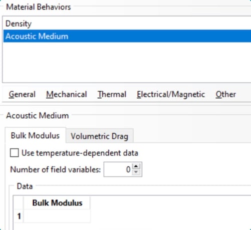
Optionally, a volumetric drag coefficient can also be defined in FTL−4 units.

*ACOUSTIC MEDIUM, VOLUMETRIC DRAG

volumetric_drag_coefficient, frequency

...

This allows for the inclusion of flow resistance forces resulting from the viscosity or porosity of the medium. Frequency dependence is supported.

Special poroacoustic models—Delany-Bazley and Delany-Bazley-Miki—are also available in Abaqus/Standard, activated via *ACOUSTIC MEDIUM, POROUS MODEL=DELANY BAZLEY/MIK. These are suitable only for SSD analyses and require keyword editing.

The CAVITATION LIMIT parameter for the *ACOUSTIC MEDIUM keyword allows you to specify an absolute fluid pressure value below which the acoustic medium undergoes arbitrarily large volumetric expansion without a further drop in pressure. This enables the modeling of cavitation (specifying the hydrostatic fluid pressure via *INITIAL CONDITIONS, TYPE=ACOUSTIC STATIC PRESSURE is required).

Boundary conditions

Three types of acoustic boundary conditions are distinguished:

• natural – not directly defined (default); they signify a zero pressure gradient in the direction normal to the boundary and zero particle acceleration in that direction (no motion in that direction)—representing a fully reflecting surface (a rigid, stationary wall or a plane of symmetry), such that acoustic energy does not leave the mesh but reflects back into it.
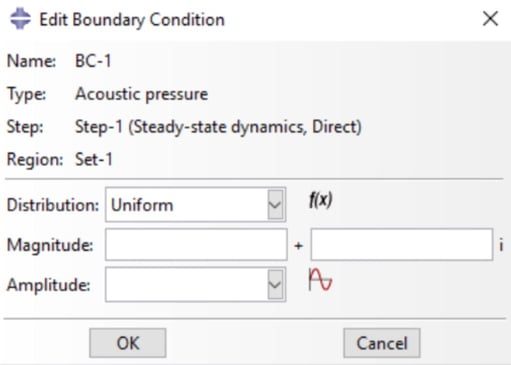
• prescribed boundary conditions – specified acoustic pressure (POR, degree of freedom no. 8, complex value in SSD analyses)
  
  • a zero value indicates a free surface (e.g., a water surface – non-zero pressure gradient, particle motion normal to the surface)
  • A non-zero value indicates a point acoustic source.
• boundary impedance representations:
  • effects of the interaction between an acoustic medium and a solid body
    (e.g., between an ultrasonic transducer head and human tissues)
  • boundaries of a fully acoustic region with known characteristics – the effect of the adjacent structure is introduced via impedance (e.g., representing a carpet in a room)
  • wave propagation conditions representing an infinite exterior acoustic domain

In direct SSD analyses, acoustic pressure is applied directly, whereas in the mode-based version, it is applied as base motion.

Acoustic impedance Z is defined as the ratio of acoustic pressure to particle velocity in a given direction: Z=p/v. Specific acoustic impedance is a property of the medium defined as Z=ρc (density × speed of sound)—the impedance of a plane wave. In SSD analyses, acoustic impedance is a complex quantity. Assigning impedance to the boundary of an acoustic mesh replaces the natural boundary condition. The acoustic impedance of a plane wave (propagating in a single direction with constant-pressure wavefronts perpendicular to the direction of propagation) is a real value, Z=ρc, and is equivalent to a viscous damper acting normal to the surface.

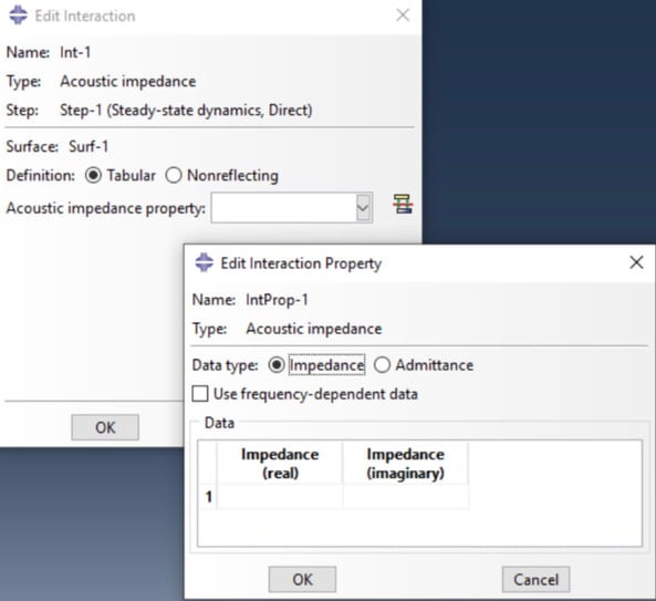
Impedance is defined in the Interaction module of Abaqus/CAE. It is assigned to surfaces. It must be specified for every step in which it is active (it does not propagate from step to step).

*SIMPEDANCE, PROPERTY=...

surface_name

or:

*IMPEDANCE, PROPERTY=...

elset, impedance_type

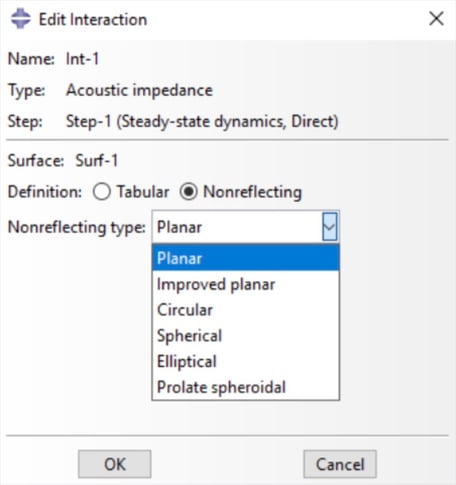
Various types of impedance conditions are available for external acoustic domains—specifically, non-reflecting (absorbing) boundary conditions for various classical wave types: plane, circular, spherical, elliptical, and spheroidal.

A tabular definition (the Tabular option) is also available, with optional frequency dependence. Instead of impedance (comprising real and imaginary parts), one can specify admittance (the reciprocal of impedance, also complex-valued). This allows for the modeling of certain loss effects occurring between the acoustic medium and a solid body (or rigid wall)—representing, for example, coatings, linings, or carpets—by specifying the interface impedance. Boundary behavior is then represented as a spring and a damper connected in series between the acoustic boundary and the solid body or substrate. For the Tabular option, an interaction property must also be created:

*IMPEDANCE PROPERTY, DATA=IMPEDANCE/ADMITTANCE, NAME=...

...

In the case of admittance, the specified values ​​are essentially the reciprocals of the spring stiffness (imaginary part) and the damper's damping coefficient (real part). In the keyword interface, the imaginary part of the admittance is specified first.

Data for multiple frequencies is required (even if the values ​​are identical across them) to enable Abaqus to accurately convert the tabular impedance parameters into admittance (thereby avoiding interpolation errors).

Acoustic loads

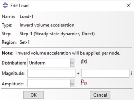
A discrete nodal acoustic load represents a volumetric acceleration centered at the node's location. For example, if a flat plate vibrates vertically, transferring acceleration to the fluid, the acoustic load equals that acceleration multiplied by the plate's surface area.

An acoustic nodal load (volumetric acceleration) is specified using the *CLOAD keyword. Such a load applied to an internal node represents a point source generating spherical waves. As in solid mechanics, refining the mesh around the point source increases the pressure in that immediate area, while results further away remain correct (analogous to Saint-Venant's principle). Acoustic loads at nodes on the boundary of the acoustic mesh represent particle accelerations in the normal direction multiplied by effective nodal surface areas. Representing a uniform boundary acceleration using *CLOAD is problematic, as it would require different values ​​for different nodes (even in certain areas of uniform meshes). The units correspond to volumetric acceleration (F·L²/M).

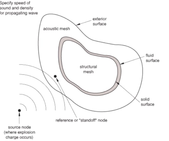
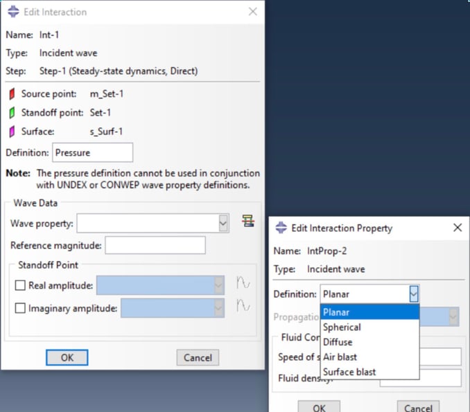
Distributed loads for acoustic elements can be applied as Incident Wave Loading (available for *DYNAMIC implicit and explicit, as well as *STEADY STATE DYNAMICS direct and subspace procedures). This involves applying a volumetric acceleration to a specified boundary surface based on a propagating wave of known form and magnitude. The source point of this wave is located outside the mesh. The following wave forms are available: planar, spherical (1/R or generalized decay), and diffuse. A reference point is also defined; together with the source point, it indicates the direction of wave propagation. Wave pressure or particle acceleration is defined at the reference point.

*ACOUSTIC WAVE FORMULATION, TYPE=SCATTERED WAVE/TOTAL WAVE

...

*INCIDENT WAVE INTERACTION, PROPERTY=...
surface, source_node, reference_node, magnitude

*INCIDENT WAVE INTERACTION PROPERTY, NAME=...
speed_of_sound, fluid_density

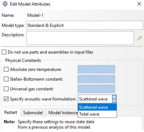
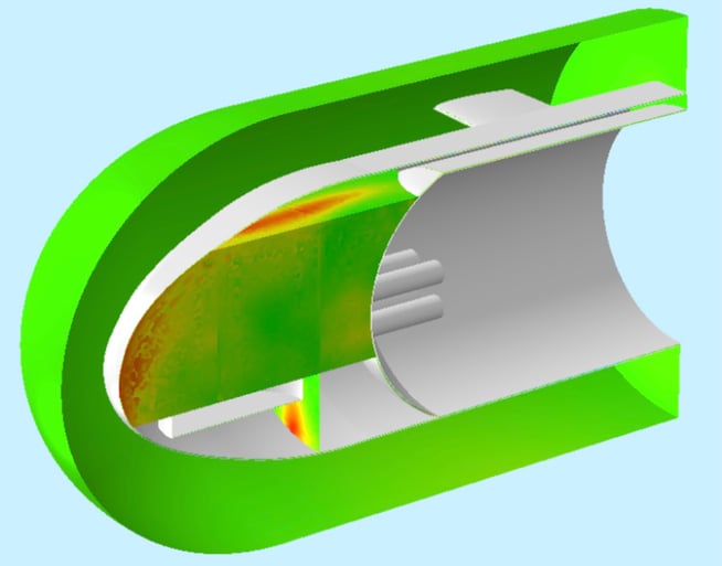
Scattering analyses are performed on structures within exterior acoustic domains featuring absorbing boundaries (impedance or infinite elements) and subjected to wave excitation originating outside the model boundaries. The objective is to determine the structural response (e.g., shock waves or microphone readings) and the scattered pressure field (e.g., sonar applications). The choice of acoustic wave formulation determines whether the solution represents the scattered wave (required for SSD analyses) or the total wave (optional for *DYNAMIC analyses). In general, the total pressure consists of two components: the known incident pressure and the unknown scattered pressure. The latter comprises a vibrational component (generated by structural vibrations) and a reflective component (resulting from the incident wave interacting with the structure as if it were rigid and stationary).

1. Scattered formulation – the acoustic pressure solution represents only the scattered component of the total pressure in the external acoustic domain (while representing the total pressure inside the structure); *DYNAMIC steps require a linear acoustic response (cavitation cannot be modeled); the Incident Wave load is applied only at the acoustic-structural interface without an interface impedance condition (not at the outer boundary of the external acoustic domain) and requires two definitions—one for the structure surface and one for the acoustic surface (representing the reflected component of the scattered pressure).
2. Total formulation – the acoustic pressure solution represents the total acoustic pressure; available only for *DYNAMIC steps and required if cavitation is simulated; the Incident Wave load is applied only to the outer boundary of the exterior acoustic domain, where absorbing boundary conditions remain active.

Due to numerical noise, the scattered formulation is recommended if the structural response is the primary focus and no cavitation occurs. With this formulation, the acoustic domain can be partitioned into two regions: one where the acoustic solution represents total pressure (near-field) and another where it represents scattered pressure (far-field). A transition zone—consisting of a single layer of linear solid elements with displacement degrees of freedom and a thickness smaller than the acoustic mesh spacing—is required to separate these two regions. This transition zone is connected to the two regions using tie constraints (the transition zone surface should serve as the master surface). The incident wave load is then applied at the interface between the transition zone and the scattered-pressure region. Infinite elements or impedance-based absorbing boundary conditions are placed at the outer boundary of this region.

Results

The primary results obtained include the POR variable (nodal acoustic pressure) and, for direct and subspace SSD, SPL (Sound Pressure Level), GRADP (acoustic pressure gradient), ACV (acoustic particle velocity), and INTEN (acoustic intensity—pressure multiplied by acoustic particle velocity). As of version 2024, the AVNSQ variable (the square of the surface-averaged normal surface velocity component, or acoustic power normalized by the acoustic impedance of the surrounding fluid) is also available for use in SSD analyses.

Energy-related outputs are also available, such as RADEN (radiated energy) and RADPOW (radiated power). If the model lacks acoustic elements, or if the goal is to calculate the equivalent radiated power on a structural surface not in contact with acoustic elements, the following can be used: ERPWR (equivalent radiated power), ERPWRDEN (equivalent radiated power density), ERPAC (equivalent radiated acoustic pressure), and ALLERPWR (equivalent radiated power emitted by a panel). ALLQB represents the energy dissipated by quiet boundaries (infinite elements). The AVNSQ and ALLQB variables allow for the calculation of acoustic power in two ways (using the plug-in listed below).

SPL (Sound Pressure Level) values ​​in dB, relative to a reference pressure, can be obtained via the keyword interface. The reference pressure is defined using *PHYSICAL CONSTANTS:

*PHYSICAL CONSTANTS, SPL REFERENCE PRESSURE=...

and:

*NODE OUTPUT

POR, SPL

Plugins are also available in the Knowledge Base that allow for the determination of additional quantities, such as acoustic power and its level (SWL), Sound Pressure Level (SPL), and Sound Transmission Loss (STL). Another plugin enables the visualization of Acoustic Contribution Factors (the contribution of each vibration mode to the total structural or acoustic response) based on calculations and their storage in the SIM file via the *ACOUSTIC CONTRIBUTION keyword. Interestingly, there is also a plugin that generates .wav files from pressure results in acoustic analyses, making it possible to “hear” them.

Grid size

The element size is related to the maximum frequency (or minimum wavelength). Higher-frequency responses require smaller elements. For reasonable accuracy, it is recommended to have at least 6 representative internodal intervals (defined as the distance from a node to its nearest neighbor within the element—i.e., the size of a linear element or half the size of a quadratic element) per shortest wavelength in the problem.

The maximum element size (internodal interval) can be estimated using the formula:

L_max < c/(n_min*f_max)

where: c=sqrt(K/ρ) is the speed of sound, n_min is the number of internodal intervals per acoustic wavelength (recommended n_min ≥ 10), and f_max is the maximum frequency in the problem.

This formula can also be inverted to determine the maximum frequency that can be captured with a given mesh.

An excessively coarse mesh may result in significant variations in the Pressure-Over-Closure (POR) relationship across elements.

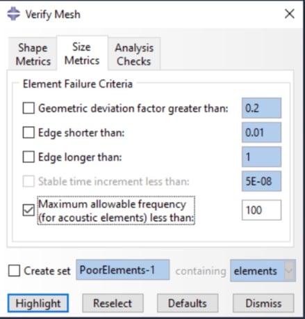
Abaqus includes a built-in check for this criterion in the Mesh module:

Domain connections

Tie constraints can connect acoustic elements to structural ones, or acoustic elements to acoustic elements from a different domain (though for greater accuracy, a mesh transition zone—roughly one wavelength of the medium with the higher wave speed—can be employed). When mesh densities are similar, the medium with the higher wave speed should serve as the "main" (master) side. The coarser interface mesh should be on the "main" side. Improper side selection can lead to a "partition effect."

The near-field is typically defined as the region within one structural wavelength of the interface; it shrinks as frequency increases. In this zone, mesh quality significantly impacts accuracy. Element size on both sides of the interface is dictated by the medium requiring the finer mesh. Beyond one structural wavelength lies the far-field.

The selection of structural-acoustic interface meshes depends on the shortest wavelength. At low frequencies, the structural wavelength is significantly shorter than the acoustic one, so it governs the interface mesh. Meshes from both domains should have comparable densities near the interface.

Structural-acoustic coupling can be implemented using ASI (acoustic-structural interface) elements. These elements activate coupling if the structural and acoustic meshes share nodes. ASI element normals must point toward the acoustic medium. Impedance boundary conditions can also be defined on the acoustic surface. In Abaqus/CAE, ASI elements are created as "skin" elements, with the "Modeling intent" in the "Element Type" dialog set to "Interface" for acoustic elements. However, a surface-based approach is recommended (as an alternative to acoustic submodeling); it does not require the manual creation of ASI elements and utilizes tie constraints. These constraints generate ASI elements internally and do not require mesh continuity. In this case, impedance conditions can also be applied to the acoustic surface. The normal vectors of the structural and acoustic elements must point toward each other. The material with the lower wave speed should have a finer mesh and be defined as the secondary surface. If solution details at the interface are critical, the meshes on both sides should have the same level of refinement, satisfying the requirements for the material with the lower wave speed. Boundary conditions can be applied to degree of freedom 8 at the nodes of the acoustic mesh.

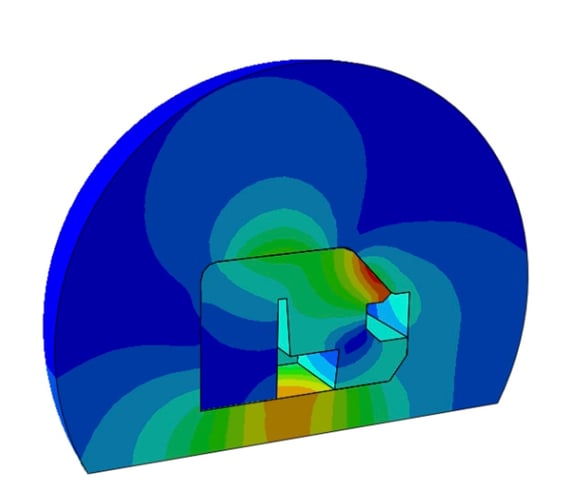
Sequentially coupled analyses are suitable when the pressure exerted by the fluid has a negligible effect on the structure (e.g., a vibrating machine radiating sound into the air, where the reactive air pressure has little impact on the machine). A structural analysis is performed first, and its results drive the acoustic analysis. This is facilitated by the submodeling technique. The global model is a structural analysis (containing only the structure), while the submodel is a purely acoustic analysis featuring ASI elements at the interface (with their nodes driven by the submodeling process). The acoustic domain mesh does not need to match the structural mesh. In the submodel analysis, the following are defined:

*SUBMODEL, EXTERIOR TOLERANCE=...

nset

*BOUNDARY, SUBMODEL, STEP=...

nset, 1, 3

Another application of submodeling in acoustics arises when the structural response is the primary focus, and the presence of a (heavy) fluid is required mainly to apply a load to the structure. In this case, the global model is a coupled structural-acoustic analysis, while the submodel is an uncoupled structural analysis. Interpolated acoustic pressures are converted into concentrated loads.

*SUBMODEL, ACOUSTIC TO STRUCTURE

surface

*BOUNDARY, SUBMODEL, STEP=...

nset, 8

Issues involving external acoustic domains

Three methods for modeling infinite boundaries are available in Abaqus:

• non-reflecting impedance boundary conditions – accurate only for plane waves incident normally on flat boundaries (in other cases, they are merely an approximation, with waves transmitted across the boundary with slight reflection); Abaqus calculates the appropriate impedance for the selected wave type, or it can be defined directly (though calculation is possible only for objects with regular shapes); in SSD analyses, they automatically account for frequency dependence.
• Perfectly Matched Layers (PML) - artificial absorbing layer used to shorten the infinite domain (only for direct SSD analysis)
• infinite acoustic elements - more accurate than impedance conditions (but higher computational cost), sometimes they can even be applied directly to the structure, eliminating the meshing of the external acoustic domain

Non-reflecting impedance boundary conditions yield highly accurate results when the model boundary is sufficiently far from the acoustic source. At large distances, all impedance formulations converge to plane-wave conditions. A good rule of thumb for the distance—applicable to more complex wave types (such as spherical, cylindrical, or elliptical)—is to place the boundary at a distance of half the structure's longest characteristic wavelength; in some cases, one-third suffices. It may be advisable to conduct separate analyses for low frequencies (requiring a larger geometric model and coarser nodal spacing) and high frequencies (allowing the boundary to be closer to the structure). Different types of impedance boundary conditions can be applied at various locations within the acoustic domain (e.g., a cylindrical region with hemispherical ends might employ both cylindrical and spherical conditions):

*SIMPEDANCE, NONREFLECTING=CIRCULAR/SPHERICAL

surface, boundary_radius

or:

*IMPEDANCE, NONREFLECTING=CIRCULAR/SPHERICAL

elset, impedance_type, boundary_radius

For plane waves in the *DYNAMIC procedure (implicit or explicit), the "Improved planar" option can be used; this provides accurate conditions for oblique angles of incidence.

The Perfectly Matched Layer (PML) functions similarly to other approaches but handles steeper angles of incidence and requires a minimum of 4–7 element layers to represent the infinite domain. It is capable of absorbing waves across a range of frequencies. The user specifies the coefficients defining the layer's absorption properties and the outer limits of the acoustic domain. The boundaries of both the acoustic domain and the PML must be rectangular (in 2D) or parallelepipedal (in 3D). The PML extends outward from the specified starting point.

*PERFECTLY MATCHED LAYER, TYPE=CARTESIAN, NAME=..., ELSET=...

PML diagonal point coordinates

*PML COEFFICIENT, VARIATION=LINEAR

...

This option is not supported in Abaqus/CAE. The PML coefficient is related to the attenuation constant describing exponential decay. Values ​​that are too low result in reflections from the zero-pressure boundary, while values ​​that are too high cause reflections from the interface with the PML region. It is recommended to select the coefficient η for a PML layer of thickness H such that: 8 <= (ηH)/4 <= 32.

Infinite elements (ACIN) are more accurate than non-reflecting boundaries. They can replace a significant portion of the outer acoustic domain mesh. They possess surface topology, and their normal direction must point outward. A reference point must be located behind the element surface. Lines extending from this point through the element nodes form "nodal rays." The angles between these rays and the element normals should be minimized. A spherical surface with the reference point at its center yields the best results. The default condition on the outer ("infinite") side is symmetry, though impedance or coupling to other elements can also be defined. This is achieved by defining surfaces based on the outer faces of the infinite elements and using the *SIMPEDANCE or *TIE keywords.

Creating acoustic infinite elements in Abaqus/CAE:

1. Creating a shell part or importing a shell mesh.
2. Assigning a reference point in the Part module.
3. Creating and assigning an "Acoustic infinite" section.
4. Ensuring that normal directions point away from the solid domain and toward the infinite domain.
5. Assigning "Acoustic" elements with an "Infinite" modeling intent in the Mesh module.
6. Attaching the infinite elements to the model using tie constraints.

An alternative method using skins:

1. Creating a reference point for the solid body to serve as the center of the infinite domain.

2. Creating a skin on the geometry/mesh (Special --> Skin --> Create).

3. Assigning the “Acoustic infinite” section to the skin.

4. Checking the normal directions for the skin (Assign --> Element Normal).

5. Assigning “Acoustic” type elements with an “Infinite” modeling intent.

Several special variables are available for ACIN elements for debugging purposes, as well as the acousticVisualization script (accessible via the `abaqus fetch` command) for visualizing far-field results on them.

Example

As an example, consider a steel cantilever beam with dimensions of 5 × 20 × 200 mm. Its first natural frequency (in a vacuum) is 100.08 Hz (analytical value: 103.46 Hz). If we place this beam in water modeled as an external acoustic domain, the first flexural vibration frequency drops to 84.287 Hz.

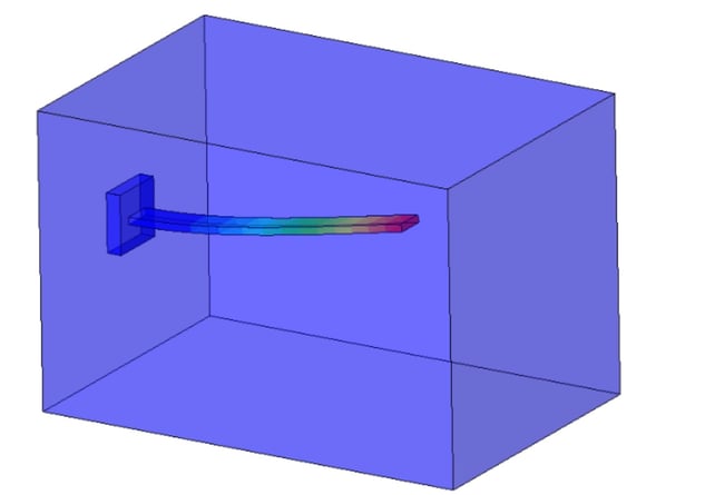
As an example, consider a steel cantilever beam with dimensions of 5 × 20 × 200 mm. Its first natural frequency (in a vacuum) is 100.08 Hz (analytical value: 103.46 Hz). If we place this beam in water modeled as an external acoustic domain, the first flexural vibration frequency drops to 84.287 Hz.

Summary

Abaqus offers extensive tools for acoustic and coupled (one-way or two-way) acoustic-structural analyses. In addition to standard acoustic elements, infinite elements and elements for modeling the fluid-structure interface—most easily created automatically using tie constraints—are available. Impedance boundary conditions (including non-reflecting conditions for various wave types) and incident wave definitions are also supported. Acoustic analyses can be performed using a range of linear and nonlinear dynamic procedures (including explicit dynamics). Modeling shock waves in air or water is also possible; however, it should be noted that acoustic behavior is typically linear unless cavitation is modeled.

Further information on these topics can be found in the documentation, starting with the "Coupled Acoustic-Structural Analysis" chapter. We also encourage you to take the "Structural-Acoustic Analysis Using Abaqus" training course.