When you build a model in Dymola, you rarely think about the equation form. You drag components, connect flanges, and press simulate. But Dymola offers one setting that can change your simulation time by a factor of fifteen, and most users never touch it.
This article explains what that setting does inside the solver, and how to decide.
ODE and DAE in one minute
An ODE (ordinary differential equation) directly tells us how a variable changes with time:
der(x) = f(x, t)
A solver moves forward by repeatedly asking: "What is the current value and how fast is it changing?" With an ODE, the answer is direct. The current values are used to calculate the derivatives, and the simulation continues.
A DAE (differential-algebraic equation) also includes equations that must always be satisfied:
F(der(x), x, y, t) = 0
This is the short form. Written more openly, a DAE has two parts:
der(x) = f(x, y, t) differential equations
0 = g (x, y, t) algebraic equations
The main difference is y. These variables do not have their own differential equation. Their values are found from the equations and constraints in the system.
For example, the force in a rigid rod is whatever value is needed to keep two connected bodies together. We do not calculate a derivative for this force. Instead, we calculate the force that satisfies the constraint. Because of these extra constraints, a DAE cannot always be written in the simple form der(x) = f(x) like an ODE.
Every Modelica model starts as a DAE
This is not a modelling choice. Modelica models are written as equations, and these equations are not always ODEs. Connections between acausal ports show this clearly. A flange connection gives two equations:
s_a = s_b positions are equal
f_a + f_b = 0 forces are balanced
These equations connect two components, but they do not say which side calculates what.
Dymola solves this during translation, before the simulation starts. It removes extra variables, sorts the equations and breaks loops where it can. The result is a set of states and a calculation order, which is often very close to an ODE. This is why an ODE solver like Cvode can simulate a Modelica model.
But some loops cannot be removed and stay as algebraic systems. With an ODE solver, Dymola must solve these loops again at every step; nonlinear loops need an iteration, linear ones are solved directly. The size of the nonlinear part is what matters when you choose a solver.
Solver settings
Open Simulation → Setup. Two settings are important.
The first is the solver type. Dassl, Radau IIa, Esdirk, and Ida are DAE solvers, while Cvode, Dopri, Euler, and fixed-step solvers are ODE solvers. The default is Dassl.
The second is DAE mode:
Advanced.Simulation.Define.DAEsolver = true;
This option must be enabled before translating the model.
When DAE mode is off, Dymola solves the remaining algebraic equations internally. When it is on, these equations are passed directly to the DAE solver and solved together with the states.
Three test models
To show when DAE mode makes a difference, three very different models are used.
Model A is a chain of n masses connected by springs and dampers. Each mass has its own state, and there are no algebraic constraints.
- Continuous-time states: 200 (n = 100)
- Nonlinear systems after translation: none
Model B is a manifold with n parallel pipes connected between two junctions with no volume. Since the junctions have no pressure state, their pressures become algebraic variables. As a result, the flow in each branch depends on all the others.
- Continuous-time states: 2 (n = 32)
- Nonlinear system after translation: {98}
- Linear systems after translation: none
- Nonlinear systems after translation: {2, 2, 2, ...} (32 small loops)
Model C is a tank that is filled with water through n valves. Each valve opens and closes 25 times per second, but the valves take turns, so the total flow into the tank is almost constant. After each valve there is a short pipe, and between the valve and the pipe there is no volume. So the flow in each branch is found from the valve and the pipe together: one small nonlinear loop for each branch
Continuous-time states: 2 (n = 32), the water level and the temperature in the tank
Results
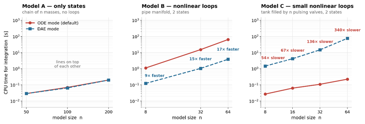
Figure 1 — CPU time against model size.
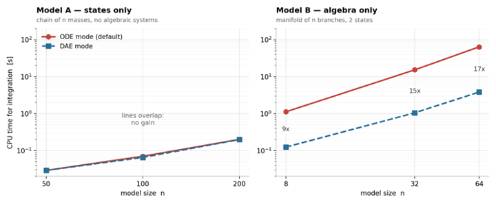
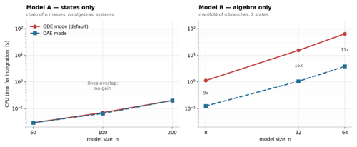
For Model A, the two results are almost identical. DAE mode is active, but there are no significant algebraic equations for it to solve, so the performance is unchanged.
Model B is different. At n = 64, the solver accepted 148 steps in ODE mode and 114 steps in DAE mode, which is relatively similar. This shows that DAE mode does not take fewer steps through time. Instead, it reduces the work required in each step, making the simulation faster.
Model C is the opposite: DAE mode is 54 to 340 times slower. The two states, the water level and the temperature, change slowly. In ODE mode the solver only follows these two states, so it needs only about 20 steps for 10 s. The flow in each branch is calculated inside each step. In DAE mode the branch flows are also given to the solver, and they go up and down 25 times per second. The solver must follow every wave, so it needs 50 000 to 68 000 steps. The result is the same, it only takes much longer.
When DAE mode is not a good idea
- The model has no nonlinear loops, or only small ones (Model A, Model C). Linear loops are solved directly in both modes. There is no gain, and it can even be much slower.
- Some values change much faster than the states (ripple, vibration, switching). DAE mode must follow them.
- The model runs in ODE mode but fails in DAE mode. This can happen, because all algebraic variables need good start values.
- Translate the model and check "Sizes after manipulation of the nonlinear systems". If the result is { } or {1, 2}, DAE mode is unlikely to provide any benefit, and it can even be slower. If the size is around {25} or larger, it is worth testing.
- Enable DAE mode before translation.
- If you enable DAE mode, test different solvers again. The default solver, Dassl, is not always the best choice for every model.
- Always compare with ODE mode. If DAE mode is slower or fails, go back to ODE mode.
How to decide
- Translate the model and check "Sizes after manipulation of the nonlinear systems". If the result is { } or {1, 2}, DAE mode is unlikely to provide any benefit, and it can even be slower. If the size is around {25} or larger, it is worth testing.
- Enable DAE mode before translation.
- If you enable DAE mode, test different solvers again. The default solver, Dassl, is not always the best choice for every model.
- Always compare with ODE mode. If DAE mode is slower or fails, go back to ODE mode.

 Engineering