Abaqus/Standard and Abaqus/Explicit Co-Simulation

What is Co-Simulation?

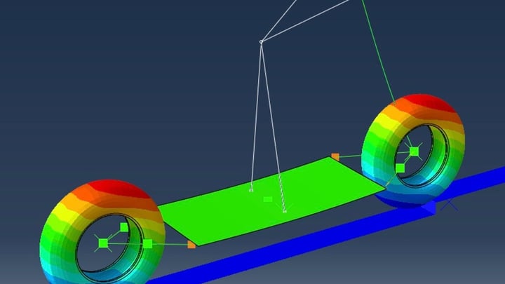
Abaqus features specialized tools that enable co-simulation, which refers to analyses where different solvers are coupled together during runtime. Most frequently, this involves Abaqus and another simulation program. However, it is also possible to couple two Abaqus solvers. The SIMULIA Co-Simulation Engine supports the following types of co-simulation:

• Fluid-Structure Interaction (FSI) – coupled fluid and solid analysis – fluid flow computed on the 3DEXPERIENCE platform, inXFlow, or other CFD software.
• Conjugate Heat Transfer (CHT) – heat transfer between a flowing fluid and a solid – fluid flow computed on the 3DEXPERIENCE platform or other CFD software.
• Electromagnetic-Thermal or Electromagnetic-Mechanical Coupling – Abaqus/Standard coupled with itself, CST Studio, or other electromagnetic analysis software.
• System Modeling – physical and logical components, Functional Mock-up Interface – e.g., with Dymola.
• Coupling with MBD (Multi-Body Dynamics) Simulations – Simpack.
• Interaction between Implicit and Explicit Dynamic Analysis.

Applications of Standard-Explicit Co-Simulation

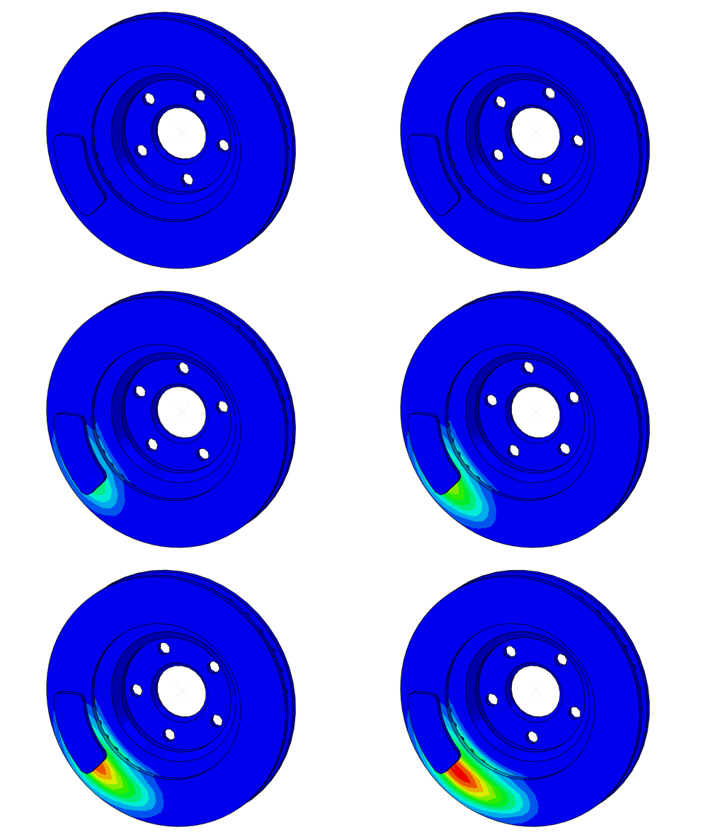
This article discusses the latter type of co-simulation: coupling Abaqus/Standard with Abaqus/Explicit. Its purpose is to leverage the advantages of both solvers within a single model. Abaqus/Standard is unconditionally stable, efficient for moderately nonlinear analyses (relatively small deformations and mild contact conditions), and allows the use of substructures. On the other hand, Abaqus/Explicit excels at highly nonlinear problems (large deformations, complex contact conditions) and high-speed dynamics.

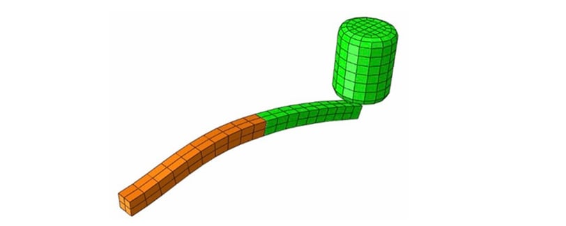
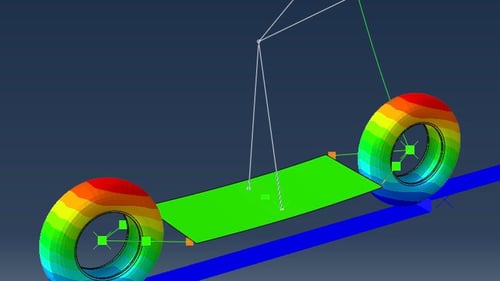
Thanks to co-simulation, a model can be split into a part solved using the Standard solver and a part solved using the Explicit solver. Naturally, these regions are selected to exploit the aforementioned strengths of each solver. For instance, a vehicle in a head-on collision can be partitioned into the front section - where contact and significant deformations occur - and the rear section, where such conditions are absent and deformations are relatively small. The computation will be more efficient in Explicit for the front and in Standard (implicit) for the rear of the vehicle.

Fundamentals of Standard-Explicit co-simulation implementation

Both parts of the model must be defined separately – in separate .inp files or CAE models. The co-simulation region is defined as the surface or set of nodes where the interaction between the solvers occurs (the connection between both parts of the model). The meshes on both sides of this connection can be non-matching (discontinuous) if element-based surfaces defined on linear elements are used. Sometimes, the stability and accuracy of the solution can be improved by matching the interface nodes. Two schemes for controlling time increments are available:

1. Lock-step – forces Abaqus/Standard to match the time increment sizes in Abaqus/Explicit - small increments in Abaqus/Standard, low memory overhead, displacement compatibility in the connection region, a good method for cases with a large number of interface nodes and relatively small models in Abaqus/Standard,
2. Subcycling – allows the increment sizes in Abaqus/Standard to differ from the increments in Abaqus/Explicit - large increments in Abaqus/Standard, computationally expensive solving of the interface, velocity compatibility in the connection region, a good method for cases with a small number of interface nodes.

Substructures allow for further reduction of the computational cost of co-simulation if certain parts in Abaqus/Standard can be treated as linear. When the retained nodes of a substructure are part of the co-simulation interface, these regions must be node-based.

Defining Standard-Explicit Co-Simulation using keywords

1. Creating 2 .inp files – one for each part of the model. The same step time must be defined for both files, and it is important to remember that the NLGEOM parameter is active by default in Abaqus/Explicit, but not in Abaqus/Standard.
2. Activating the co-simulation – using the *CO-SIMULATION keyword.
3. Defining co-simulation regions (interface) — keyword *CO-SIMULATION REGION (TYPE=SURFACE or NODE). The required designations for exchanged solution fields depend on the co-simulation method and are described in the Structural-to-Structural Co-Simulation documentation section

1. Running the analyses, considering optional import from Abaqus/Standard to Abaqus/Explicit.

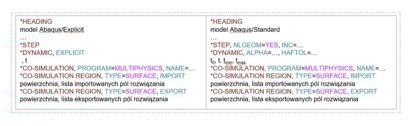
Below is a template of .inp files for a Standard-Explicit co-simulation:

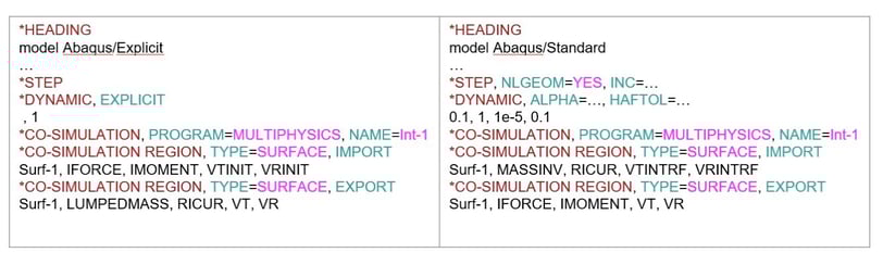
Example keywords for the subcycling method:

Defining Standard-Explicit Co-Simulation in Abaqus/CAE

1. Assemble the components for Abaqus/Standard and Abaqus/Explicit within a single model, but as separate parts.
2. Copy the model to create one model for Abaqus/Standard and one for Abaqus/Explicit.
3. Optionally, link instances across both models (Link Instances option) – this helps visualize the entire model, and linked instances are updated automatically. Exclude the Standard model instance from the Explicit model, and vice versa.
4. Define steps – dynamic, explicit and static or dynamic, implicit.
5. Define loads, boundary conditions, contact, constraints, output requests, and other analysis features in both models. To animate results from both analyses simultaneously, field output must be saved at identical time frames in both analyses.
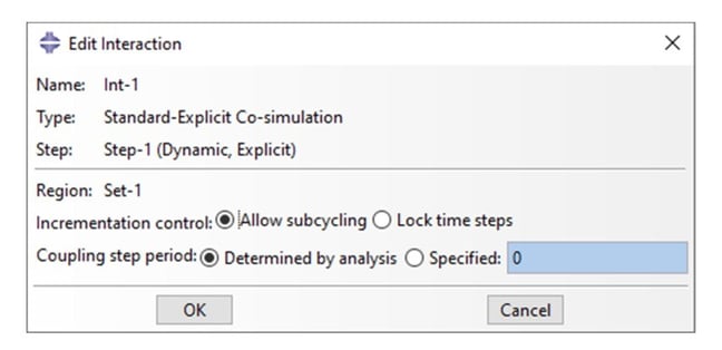
6. Create a Standard-Explicit Co-simulation interaction and select the time incrementation control method. It is not recommended to use the Specified setting for the Coupling step period – this will lock the increments in Abaqus/Explicit to the entered value. If these increments exceed the stable time increment, the results may be incorrect.

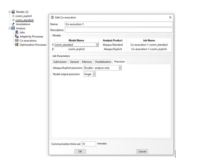
7. Create and run a Co-execution. Double precision is recommended for Abaqus/Explicit, and separate CPU cores should be allocated to individual parts of the analysis.

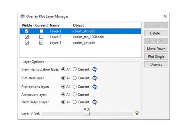
8. The co-simulation generates separate .odb files – one for Abaqus/Standard, one for Abaqus/Explicit, and one for each substructure used in the Abaqus/Standard analysis (if substructures are utilized). To display the results of both analyses simultaneously, Overlay plots can be used. When opening files, check the Append to layers option. These plot settings are managed via the Overlay Plot Layer Manager. Settings such as the deformation scale factor, the legend (manually defined limits), and the displayed variable should be identical across layers. All layer options should be set to All so that changes are applied to all layers simultaneously. If the number of frames differs between the two analyses, a Time-based animation can be used to synchronize them.

Modeling tips

1. Co-simulation requires a configuration file (XML), but in most cases, it is generated automatically (by Abaqus/CAE or from the parameters of the *CO-SIMULATION keyword). Certain advanced cases require manual definition of the configuration file based on ready-made templates or so-called elaborated configuration files.
2. An enhanced subcycling method is also available. It provides robust and accurate solutions for strongly coupled physical problems and is preferred for this type of co-simulation.
3. Avoid defining constraints within the co-simulation region (interface). Constraints on the Abaqus/Standard side will cause an error, while on the Abaqus/Explicit side, they jeopardize solution compatibility (the effect may be negligible if only a small fraction of interface nodes have constraints defined).

Additional performance optimization methods

1. Utilizing substructures in Abaqus/Standard.
2. Solving parts of the model with small time increments in Abaqus/Standard.
3. Minimizing the size of the co-simulation interface – ideally to several dozen nodes.
4. Reducing the model size in Abaqus/Standard.
5. Increasing the ratio between increment sizes in Abaqus/Standard and Abaqus/Explicit (ideally > 50).
6. Avoiding substructure output recovery for a large number of output frames – this can extend computational time by up to 15%.

Summary

Abaqus enables co-simulation not only with external software (to solve coupled and multi-domain problems) but also between the Standard and Explicit solvers themselves. Such analyses allow users to exploit the benefits of both solvers concurrently. Abaqus/Standard allows the use of substructures and is more efficient for static and dynamic problems without severe nonlinearities, whereas Abaqus/Explicit is more efficient for quasi-static and dynamic problems involving strong nonlinearities, including severe contact conditions. Co-simulations are characterized by a significantly lower computational cost compared to analyses performed entirely in Abaqus/Explicit. This cost can be further reduced through the use of substructures.