Stability Analysis in Dymola

This article introduces several ideas that provide foundations for stability analysis in DYMOLA.

Those ideas have several applications, including the creation of root locus diagrams, which provide information about transient behaviour (and therefore stability) and assessment of frequency-response that details how well an input is translated to an output, in terms of the constituent frequencies of the input.

The methods illustrated have most bearing on controller design & signal processing, in practice – but initially, simpler systems which contain no feedback will be examined to maintain the greatest simplicity.

It will also explain the nature of linear feedback. Models laid out intuitively in the DYMOLA GUI are connected systematically with the ideas of Laplace-domain block diagrams commonly used in controller development, while the concepts of proportional, integral & differential control are briefly summarised.

Ideas used to carry out stability analyses will hopefully become more easy to connect with the computer models, with the relationships between alternative system representations clarified.

In this article, DYMOLA computes outputs from a single example system, subjected to a step input. Advantage is taken of the flexibility of the DYMOLA environment.

Finally, we will explain the nature of a root-locus diagram, and how to create one using the DYMOLA software.

The DYMOLA software includes considerable professionally engineered, largely open-source tools for stability analysis, including inbuilt linear analysis toolset & the contributions by Europe’s premier aerospace research centre Deutsches Zentrum für Luft- und Raumfahrt e.V.

Why Use Dymola for Stability Analysis?

As Dymola can easily redefine the known & unknown quantities in models without modification to the model architecture, and because the software can linearise the dynamical system in a fast & appropriate way, the assessment of stability characteristics in Dymola can be quick, effective & accessible to non-experts in CAE / coding, or those simply unfamiliar with (parts of) the model.

Occasionally it is suggested that the speed & effectiveness of the software is not critical, due to the power of modern computing. However, if one considers the use of Design of Experiment approaches one may need a large number of (possibly sequential!) model executions & the convenience of having software that does not require a high-spec workstation.

So: Running in 2sec rather than 5sec is significant!

Effectiveness in Modelling

Dymola can:

• Easily redefine the known & unknown quantities in models without modification to the model.

• Linearise the dynamical system in a fast & appropriate way.

• Construct root locus & other useful illustrations, without the user needing to have (complete) knowledge/understanding of the model – in sharp contrast to many other engineering tools.

• Plot root loci quickly, without restricting itself in terms of the form the model equations take, or what parameter it’s possible to vary as “K”.

• Flex between causal & acausal modelling, or combine the two, to:

  • Create the best possible environment for controller design

    • Within DYMOLA alone, or via interface with other software

    • Possibly using items of controller-in-the-loop hardware

  • Avoid using controller-development “block diagram” tools for modelling physical systems.

    • DYMOLA using controller-development “block diagram” tools for modelling physical systems.

    • Modelling a physical system using causal controller blocks is far from ideal!

Model Based Systems Engineering

The modular structure of Dymola lends itself to incrementally adding features & details. Testing to make sure the model still works as expected is also easy. These qualities serve Systems Engineering which requires documentation of how models are developed & results reached, in order to accurately and easily adjust those models as ideas develop, or are revised.

In short, when using model based systems engineering, it is critical to be resistant to error, and for models to be reusable and flexible.

The principles of RAMSii apply to models & processes for modelling, as well as the final product.

Representing a Plant Model

In this section we establish transfer functions as a way to characterise a physical system. We observe that there are theorems which let us judge the stability based on certain qualities of these functions.

Map of a Simple Dynamical System

We begin with the RC circuit discussed in the ‘A State-Space Model of simple RC Network in Dymola & potential Applications’ blog post to illustrate¹.

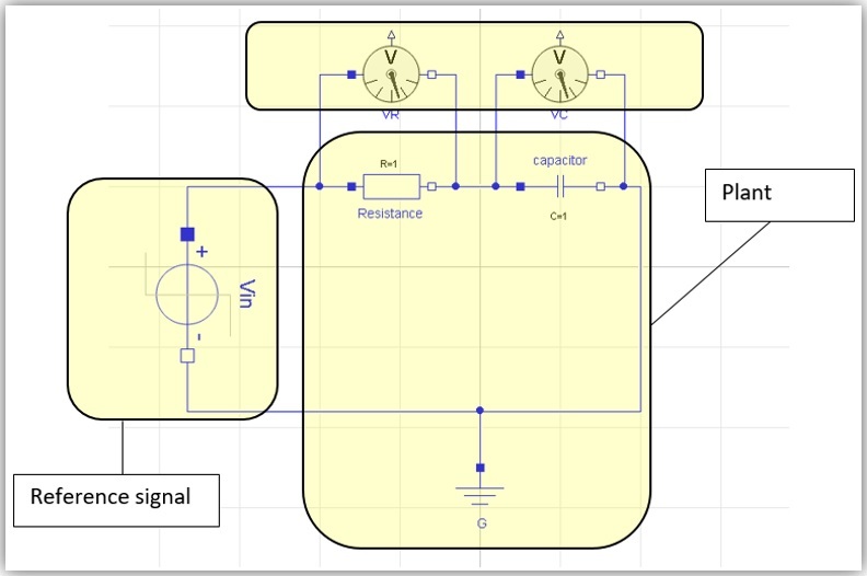
Figure 1: Model in DYMOLA GUI divided into different parts of a control architecture

Transfer Functions

Transfer functions describe the way in which an output signal responds to any input signal. They contain a complex variable, giving insight into both amplitude and phase² of the output relative to the input. Transfer function just means:

“how an output responds to an input”

In principle the output might not respond at all (transfer function  0) or it might mean ‘exactly’; i.e. the input comes straight out precisely as it came in, (transfer function  1). Under many circumstances, though, the output might (amongst other properties) lag significantly behind the input. This creates scope for control systems that act too late, and therefore counterproductively.

Transfer functions describe the response using the complex variable that results from using the Laplace transform. In the Laplace domain, common inputs, like a step function, correspond to algebraic (and continuous) functions, as do linear operators like differentiation.

Because of these properties, block-diagrams can be created, and simplified to illustrate what is going on, then converted back to the time-domain. As with many aspects of control by the transfer function approach, one important advantage of this is just “visualising” & being able to work intuitively, using simple arithmetic operations.

Transfer functions contain useful information about:

1. The transient response
2. The steady-state response

• It can be a challenge to ensure the initial behaviour of a system after a sudden input (gust of wind, impact by an object, wave, puddle) is satisfactory.
• Unstable outputs are a form of transient outputs which grow, instead of dying away.

Laplace Representation

We now return to the simple example of the RC circuit in Figure 1 and reach the Laplace domain transfer function of the system for now, without any feedback or other extra complications.

Take the equations relating the quantities of interest:

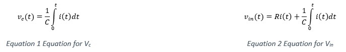
The goal is to find a characterisation of the ratio of a reference signal to a chosen output. We apply the Laplace transformation with the assumption of zero initial conditions. If you are not already familiar with this integral transform, note that integration becomes 1/s.

We can divide Equation 3 by Equation 4.

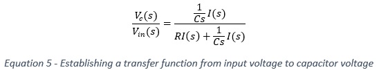
By multiplying both numerator & denominator by Cs and eliminating I(s) we simplify the expression.

Stability: Poles (Roots) of The Transfer Function

What is a Pole

From a transfer function one can factorise the denominator & create a sum of terms using partial fractions (Stewart, 2015). The separate terms can be easily transformed back into the time domain.

After partial-fraction expansion, the transfer function becomes terms that each have a linear factor like (s + 3) or an indivisible quadratic factor (s² + 1), or a “repeated factor” as the denominatore³ like (3s + 1)³. From middle-school algebra we know these factors point us to roots, also known as poles.

For the above, we refer to a “pole” at s=-3+0j for the (s+3) factor, a pair of complex poles at s= ±j for (s²+1) and three coincident poles at -1/3+0j for (3s+1)³.

What Poles Say About Stability

Fundamental Facts

With the help of some particularly pertinent inverse transforms we can obtain the time-dependent response to any input.

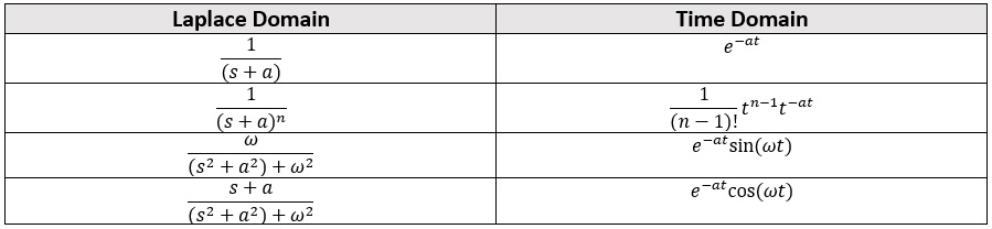
Figure 2: Some commonly needed Laplace transforms

Using this information, we observe that:

For reference, we note the final value theorem (Ogata, 2002) stating:

Review of the RC Example

The RC circuit we have constructed so far, has neither complicated behaviour, nor any feedback control system. As a result, the analysis won’t be too difficult.

What we know is:

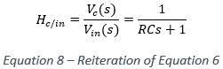
Therefore, when considering the response of  to  there is a single pole at:

This pole always has negative real parts⁴.

Unsurprisingly, the transients always die away in this system.

Getting Information from Transfer Functions

Despite the easy example, we only need to calculate the transfer function, in order to examine the transient behaviour. Consider the response with a Sine input:

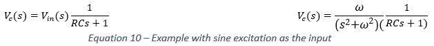
On very careful inspection, referring to our knowledge of partial fractions & the Laplace table printed in the foregoing text, one can surmise that once expanded into partial fractions & inverse-transformed:

Using Block Diagrams

Because of the conversion by Laplace Transform, linear, time-invariant physical systems or LTIs can be represented by block diagrams. Along with a scheme for systematically rearranging the blocks, this serves as a form of visualised algebra.

It is particularly useful for dealing with control systems & signals, because it is orientated towards causal systems, where a signal is sequentially operated on by processes that change the signal and pass it on.

In the world of CAE, however, some fields have arguably come to be unnecessarily dominated by such an approach, as there is little benefit in modelling the physics of machines this way, for analysis – it is simply a useful way to represent physics in the context of feedback controllers!

Block Diagram Reduction

Textbooks (Ogata, 2002), describe the simplification of block diagrams. The reader is referred to such textbooks or the resources available as online courtesy of leading technical institutions (Massachusetts Institute of Technology, 2001).

The derivation in the following section represents a simple example of this mechanistic process, which can be mastered by following a set of fairly logical⁶ rules.

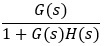
Closed Loop Transfer Function

This illustrates the use of algebra to establish the equivalent transfer function of a feedback loop. We have not yet discussed the idea of feedback, but this serves as an initial example of how we can use the block diagrams to visualise the logic of feedback controllers, for linear or linearised systems, also known as “PID” controllers (proportional, integral, differential) and available in block form in the DYMOLA libraries.

Consider a plant with transfer function G(s), with a reference input signal R(s) & output signal C(s).

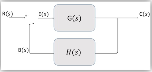
 Figure 3: A block diagram with a feedback loop to be reduced.

To reduce this diagram, we note:

Also:

Equating these through E(s) gives us:

Rearranging this leads to the form:

Because this expression shows what to expect to happen in the response, C(s) of a closed loop system under the effects of the reference input R(s) it represents the whole as a single block.

Key Points

We have established the idea of the use of the Laplace domain to create transfer functions, and the block-diagram signal approach. This opens up a way to establish equivalent transfer functions to networks of simpler functions, as illustrated above.

We have also underlined some of the ways in which the “poles” of a transfer function are significant to the transient response.

Now that we know what the location of poles means, we can look at ways to find out:

• How they change if we vary parameters in models.
• How we can use the knowledge to inform controller design.
• How we can modify the way in which we feed signals to controllers
• How to specify properties of the instruments we need to use to facilitate control.

Similarly, using knowledge of transfer functions, we will be able to partly anticipate how well periodic signals (wanted or unwanted) are transmitted, without carrying out painstaking analysis or tests, and without needing to understand coding, by way of DYMOLA’s linear analysis capabilities.

Ideas of Feedback

The meaning of a system’s “roots” was already explained in part I, but in practice, methods for stability analysis are more often concerned with systems that contain at least one feedback loop.

This is true to the degree that software for general mathematics has functions that only let you do analysis (like root locus analysis) on closed-loop systems.

It’s fair to say we don’t often need an elaborate diagram to see what the system would do when it has no feedback loop. That is mainly because there is much more limited scope for intervention (no controls). Nonetheless, the methods are entirely relevant for “open loop” systems too.

Feedback Controllers

Closed loop systems feed output information back, through certain processes, to the input. In simple examples, the output may be delivered unchanged to the input, and subtracted from the reference value (a unity feedback system) while in practice, instruments and subsystems all have a transfer function of their own, influencing the signal as it “passes through”.

The mechanism for “subtracting” the feedback signal from the reference input, like a steering servo, or aileron, likewise has its own (potentially unhelpful) transfer function. The controller itself, is only an implementation of a logical law to decide what control to apply (what command to give the servo or aileron). However, the controller is only one of many components of H(s) shown below.

Usually, the reference input represents some phenomenon outside our control,

and the controller is a mechanism that uses (our) knowledge of the plant to

compensate for the effects of the outside influence on the state (position, speed,

temperature, etc) of the plant.
 

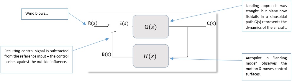
Figure 1: An example of feedback representing physics

As explained, in practice H(s) is really a product of transfer functions for:

• Instruments & sensors (which give us access to a reliable, continuous reading of what the output C(s) is.

• Controller logic (various circuitry, historically mechanical devices…)

• Signal transmission mechanism

• Actuators/Servos/Amplifiers

• Controlling device (rudder, aileron, heating element, motor, hydraulic jack)

In the diagrams below, the version on the left shows the feedback path condensed as a single transfer function, but usually H(s) will be the outcome of several terms. Using Laplace domain functions makes the process of composing and interpreting it simpler (Boyce & DiPrima, 2001).

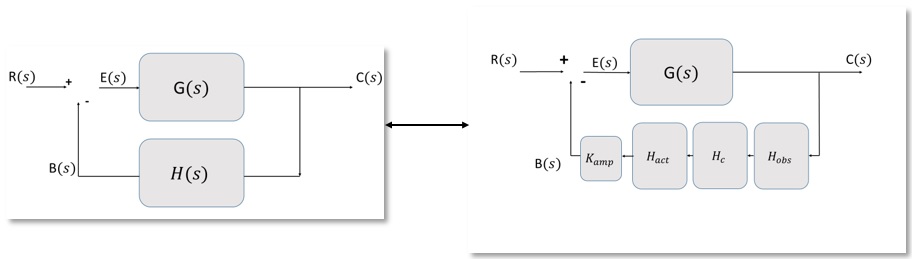
Figure 2: In practice the feedback transfer function is a product of many

Proportional, Integral & Derivative Feedback

You may have heard the term “PID” which refers to controllers that use the output itself, the derivative of the output, and the integral of the output to contribute to the feedback signal.

Each has a coefficient, called a “gain” which weights the influence of the terms.

The Laplace block diagrams help to manage the terms, especially as the integral & derivative transform to multiplication & division by s, the complex variable.

Figure 3: The above diagrams are equivalent (Ogata, 2002)

Anatomy of Feedback Control

The easiest way to show an example is to just build on the model we have been using. Here, the value of capacitor voltage is amplified processed (we will examine this later) and subtracted from the input voltage.

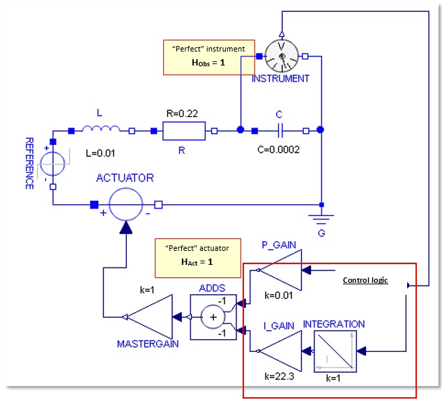
Figure 4: A closed loop system in reality includes unwanted transfer functions

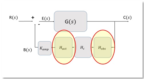
Figure 5: The transfer functions of instrument & actuator are ignored (=1)

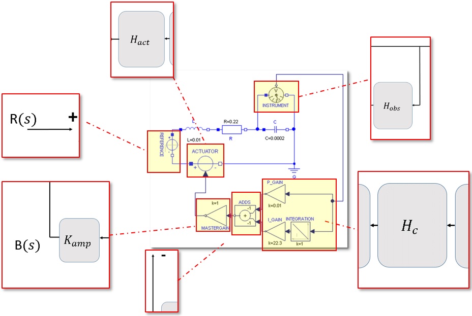
Figure 6: The simplified model leaves Hobs & Hact as unity (no effect)

Now compare the DYMOLA schematic with the block diagram containing specific functions representing the H(s) constituents. In this block diagram, Hobs(s) has been assumed to equal unity, and been left out, as has Hact(s). This matches the actual nature of the DYMOLA model shown, in which the instrument is modelled as measuring the voltage at the capacitor perfectly, and the “signal voltage” component, similarly, delivers the control signal perfectly too.

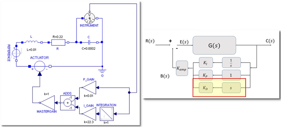
Figure 7: Dymola GUI & a block diagram separating control components as in the GUI (see also Figure 8) note that the differentiator, and derivative gain KD (indicated, right) are shown for completeness but do not exist in the GUI diagram (left)

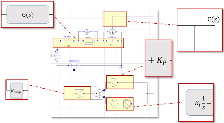
Figure 8: How the blocks correspond to the system

Example in DYMOLA

As before, we’re concentrating on the voltage across the capacitor as the output of interest. We start by illustrating the effects of feedback control, not using theory, but rather just by example results obtained by simulation. We then discuss qualitatively what the effects are, why, and what the accompanying root locus diagram will look like.

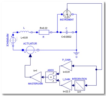
Figure 9: A causal plant with causally modelled feedback

Below, we look at the effect of proportional, and then integral control by experimenting with gain values. Note that DYMOLA easily allows us to try a range of possible values by scripting, but it also contains an arsenal of tools to analyse systems without close inspection & without advanced practical CAE skills. We’ll explore these in later articles.

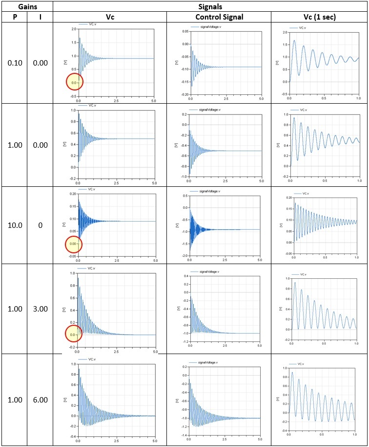
Figure 10: Selected results using a range of gains

Before proceeding we orientate ourselves with the following observation:

• The steady state response obviously depends on the reference input (Ogata, 2002) as well as the transfer function of the plant. The above is the result of a unit step input.

• The feedback control pushes the system towards zero output. The controller contains no foreknowledge of where the system “wants” to settle to.

  • Controller responds to a non-zero output (proportional) or a nonzero time-integral of the output (integral).

  • Both transient and steady-state responses due to the reference input are suppressed by the controller – it cannot “distinguish” between them, but can be “tuned” to affect some kinds of response more, or faster.

In the above diagram, we can observe the following points. These follow from examining the theory, but we have used results only to point to the effects for now. DYMOLA can quickly & efficiently generate such results. Useful for when a system is harder to examine…

With greater proportional gain (alone):

1. The system will not return to its original conditioniii (as a spring loaded by a weight – it will reach a new position, no matter how stiff).

2. One suppresses the amplitude of response.

3. Higher frequency vibrations can be generated (a stiffer spring holding your position).

If we allow integral gain:

1. Integral gain responds to the history of the output. It lets you eliminate steady state error (even a small integral gain does this eventually).

2. Integral gain arrests the average value so the signal begins oscillating around zero. The oscillations themselves are perpetuated!

3. Eventually, integral gain will cause instability. The examples show instability run longer (see diagrams!) to show the progression of the growth of the signal.
   

Most importantly we note that:

• All real control systems are limited by the strength of control signal that can be generated.
• For this reason, the control signal trace is also included!

“Maxing out” the control actuator is called “saturation” in control engineering. Bear in mind that any control schematic that treats the system as “linear” as is done here, cannot account for the fact that there is only so much control that can be applied. For example, rocket thrusters to correct course have a maximum thrust, beyond which they will deliver no more regardless of what is demanded! This is “obvious” but it is possible to become engrossed in analysis, and pay too little attention to the physical facts. It is for this reason this control “demand” has been plotted. It’s worth keeping an eye on it!

Features and Role of Root Locus Analysis

Root locus just means “the location of the roots”. Historically, a particular approach to thinking about, and constructing knowledge about these loci of the (characteristic equations’) roots was developed.

Primarily, this was a way to predict the behaviour of systems with feedback, using only the knowledge of the plant transfer function, often labelled G(s) and the feedback transfer function, often labelled H(s).

In part I, the article concluded by illustrating how to reduce a block diagram with a feedback loop to a single block. It became clear that a plant with transfer function G(s), with a feedback loop containing a transfer function H(s)i results in an overall transfer function:

  

Equation 1: The closed loop transfer function

The expression  is a form of the system’s governing equations. That expression can in many cases be factorised (part of the benefit of using the Laplace domain in the first place).

Plotting Root Loci in DYMOLA

You can use DYMOLA to plot the position of the roots of the characteristic equation, to form a series of lines called the “root locus”.

That is the core point of the concept of a root locus diagram. It is simply the locus of the roots, as they travel through the complex plane, as a result of a single parameter being varied.

Instructions for Obtaining A Root Locus Plot:

For the first example we will use the RC circuit. In this simple circuit, with no feedback and only a trivial plant model, we vary the RESISTANCE.

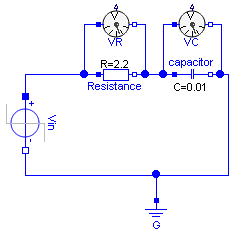
Figure 1: The simple RC circuit used 

Common sense should tell us about what kinds of things we might see, but it will prove that we’re doing things right in DYMOLA.

1. Load your model

In this example, the resistance is initially set to 2.2Ω. However, we’ve already stated that we will try a whole series of values of resistance to create the plot, so consider the following notes:

Entering a(ny) value for a variable is no problem for DYMOLA in this context. The root-locus function will supersede any value you enter in model building environment.
Though this model is linear, and very simple, in the general case, a system will be nonlinear. DYMOLA will require a “set point” around which to linearise the model. The mechanics of this are beyond the current scope. For the time-being, note that the set-point will be specifically entered in the root-locus dialogue. So, the parameter value for resistance we enter while building the model won’t be used.

The capacitance is 0.01F.

2. Go to the taskbar, click linear analysis, then root-locus analysis in the menu

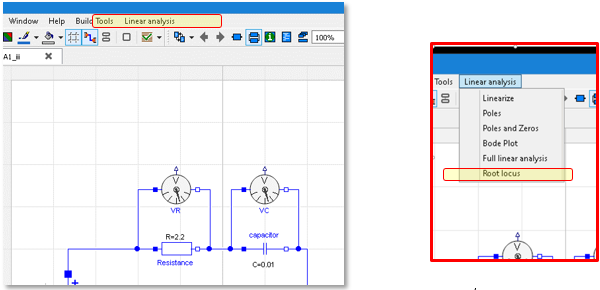
Figure 2: Selecting Root Locus from the Linear Analysis menu

3. In the dialogue, select the “tree data” tab

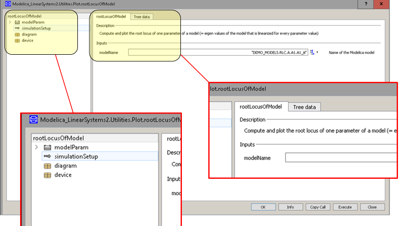
Figure 3: Find the right place to enter your parameter to vary

4. In the dialogue, click on the edit button to the right of the top dialog box–

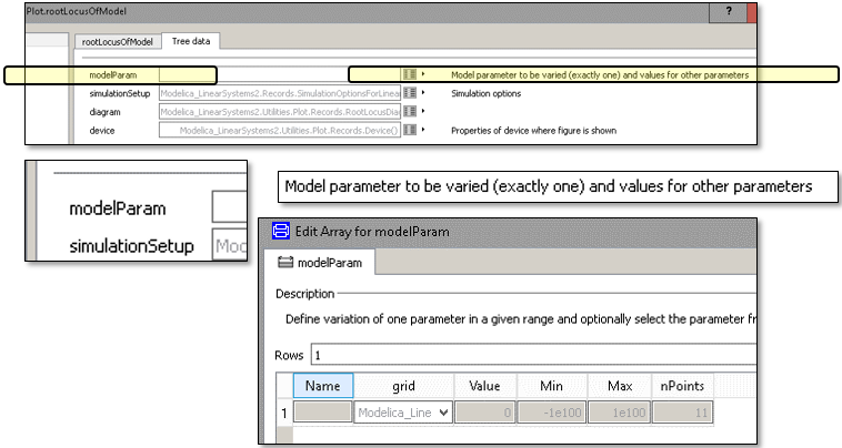
Figure 4: Reaching the parameter variation screen. The figure shows from top to bottom, the field in question (use the button to access it), a close-up of the field, and the view once the button is clicked.

5. Click the “select” button bottom right

6. Choose the parameter that you want to vary from the list displayed

7. Click OK

8. Now enter a reference value, a minimum value, a maximum value & number of values to plot. The reference value represents the expected “usual” operating point around which a system will be linearised (an already linear system will remain unchanged regardless of this value).

9. Only THEN, enter a choice for the kind of grid to be used!

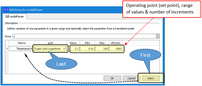
Figure 5: The values must be filled in using the right procedure & in order!

10. Click OK

11. Click execute

The resulting plot will look something like this, for the given example. It might not look like much, but you have made your first root locus plot.

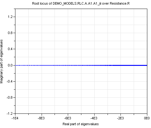
Figure 6: The simplest possible root-locus plot

The labelling of the axes by the software is deliberately left beyond the scope for the time-being but serves as a clue to the significance of the “poles” or “roots” being mapped.

Varying Inductance:

We now adopt a system (see appendices) where the resistance is set to 0.22Ω and the capacitance to 0.01F. The input voltage is a unit step.

Besides that, we also add in an inductance, which creates a voltage drop that is dependent on the rate of change of current, and therefore makes the governing equation become a second order equation.

We’ll see the root locus of a second order system is one step more complicated, because there will be two roots to track through the complex plane.

1. Run and model.

2. Select Linear Analysis in the menu bar at the top of the screen, then root locus.

3. Select the variable L, in the inductor, & values shown below.

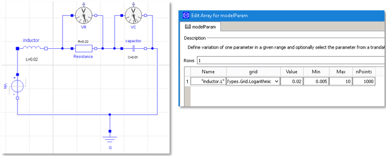
Figure 7: The “value” field is the set-point for linearisation where applicable

If you see empty space, try zooming in on the origin!

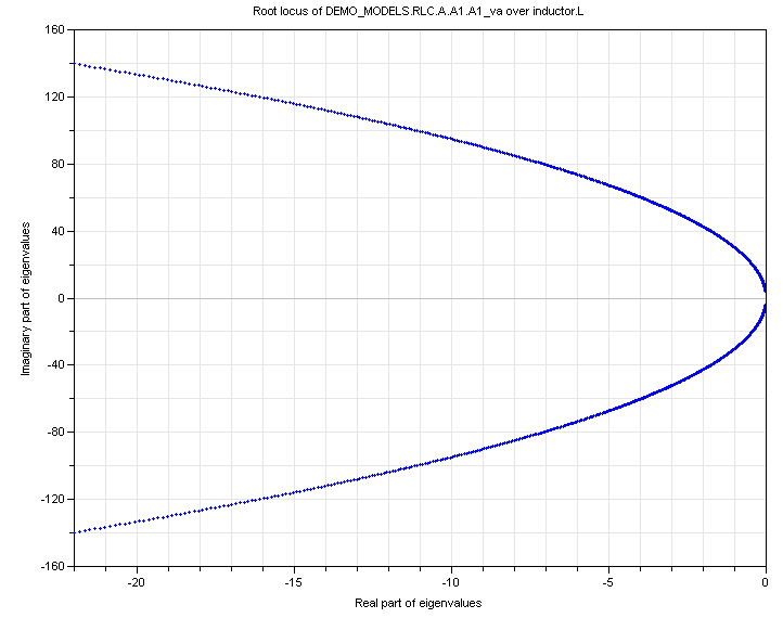
Figure 8: The position of the roots as inductance is varied

Now that it’s clear how to make the software create the diagram, the next step is to examine why this method is so useful, both originally, and today, with access to tools that can do the computations quickly.

To do that, we start from the beginning, where the root-locus approach was created.

Root Locus & Feedback Control

Computation of Roots

For the time-being, we deliberately avoid commenting on ways to find the roots of the characteristic equation. There are indeed several ways to go. In this article, one method is mentioned by name, and one is obvious from part I. A third has been mentioned in other articles, and will not be addressed here. Those are:

Evans’ method (useful for use by hand but may of course be automated).
Finding the roots of 1+GH repeatedly using a range of values for the chosen parameter (might typically use root-finding algorithms written in C++ or similar(Press & A., 2002).
Modelling using state-space ideas (uses linear algebra).
Evans’ Method 

The American engineer W. R. Evansiii devised an approach for plotting the root locus that is used to get closed loop behaviour directly from open-loop functions G(s) (plant) & H(s) (controller). We only explain the advantages & limitations here, not how to use it.

The Purpose of Evans’ Method

Evans’ method does not require the reduction of the block diagram. It is carried out using knowledge of G(s) and H(s) only. This adds insight & simplicity.

The DYMOLA user can see, by way of the diagram, what form modifications to a controller should take. However. learning to draw the diagrams by hand is very helpful in learning to interpret the result, and how to draw them, depends on Evans’ Method.

Though originally, Evan’s Method was developed to ease computation by hand, it can assist digital computation tooiv. Evans focuses on the way the roots of G(s)H(s) “contribute” to the phase lag of the feedback signal.

As a complex valued function G(s)H(s) must have phase angle 180(2k+1) and a magnitude of 1, to constitute a pole.

That is just a way to obtain roots of the characteristic equation. For control engineers or enthusiastic learners, it illustrates the sensitivity of/to a controller. Factorising the denominator of Equation 1 by algebra is avoided while automated execution avoids large numbers of function evaluations.

However:

Evans’ method (for manually drawing root loci) will not generally be useful if the characteristic equation cannot be stated in the form 1+KF(s) where F is a ratio of polynomials and K is the quantity to be varied.

To get around this limitation, one usually has to define other gains in terms of the one to be varied.

Applications

One critical and valuable area where insight is provided is when a plant exists, and a controller exists, and one hopes to modify the response, or wants to understand the effect of adding extra features to the controller.

Because the method focuses on the contributions of the terms of G(s)H(s), one can more easily guess what is going to happen.

Root Locus Analysis on a Closed Loop (“With Feedback”) System

DYMOLA – Finely Targeted Analysis vs Typical Math Software

It is important to consider that although many analysis systems allow root locus analysis, some of the most common are restricted in their utility. The most common software will carry out analysis only by varying the parameter K as shown by the form of the following diagram.

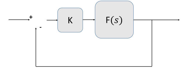
Figure 9: A prototypical “unit feedback” form of system

Bear in mind, that the root-locus will be the same for any transfer function with the same denominator. That denominator embodies the governing equations. Therefore the above diagram still results in the denominator of the transfer function becoming:

To initiate the analysis, the system has to be defined as stated above, by providing the system with the numerator and the denominator of F(s).

You then get the plot, and use it by keeping in mind that it applies to any closed loop whose transfer function has 1 + KF(s) as its denominator. Only K is varied. You cannot vary another parameter without casting it as the gain K in the above form!!

Remember, the root locus still exists for any varied parameter, and you can get that diagram from DYMOLA.

By knowing Evans’ Method though, you can reason what generalisations will and won’t apply to your system and it’s diagram.

How to implement this method – investigating and making conclusions from the behaviour of the transfer function by seeing the G(s)H(s) term a magnitude & argument is discussed in later articles.

Stability Properties of Feedback Using DYMOLA

In part II, we used the system illustrated below to explore practically what the response of a system that has proportional & integral feedback could look like. We used a simple step input (basically the simplest input that takes a nonzero value over time) and we did not look at derivative feedback.

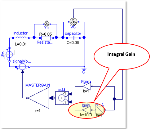
Figure 10: The feedback setup used in part II

Root Locus Plot of the Closed Loop System

We now examine the DYMOLA root locus plot. We use unit proportional gain and allow integral gain to varyv. (See section: Plotting Root Loci in DYMOLA)

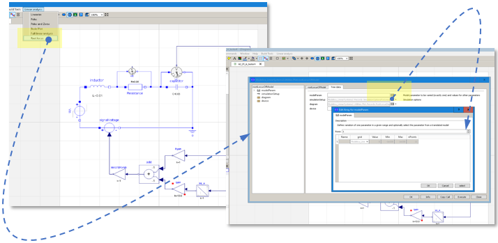
Figure 11: The diagram summarises as fast as possible which buttons you need!

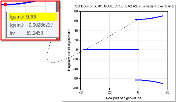
Figure 12: Using the DYMOLA GUI to spot important points on the diagram

We can see from Figure 12 where the root locus crosses the Im axis. This is also a good moment to observe that due to the nature of the controller, the closed loop system has three roots. As it is a complex conjugate pair that cross the axes, we know at a glance that there will be a growing oscillatory response (Boyce & DiPrima, 2001) if we increase the integral gain too far, corresponding to our time traces.

However, the root locus plot would show this just as clearly no matter what the reference input was, or how complicated the system. That makes it very useful, even more so now that we can construct one automatically.

Without examining how these diagrams are constructed by hand, however, it is harder to extract the full information (Ogata, 2002) from examining one. The combination of knowing in detail why various features of the diagram arise, but not needing to manually draw them is therefore ideal. Indeed, it illustrates that the knowledge of Evans’ Method is today, more relevant for interpreting these diagrams, than it is for creating them.

Final Note

Although it is useful not to be restricted in the form of model for which a root-locus diagram can be drawn, special care must be taken when interpreting diagrams for models which could not have been made by Evans’ procedure.

Such an interpretation may be useful, or even correct, but cannot be assumed to be.

References

Boyce, W. E. & DiPrima, R. C., 2001. Elementary Differential Equations & Boundary Value Problems. 7th ed. Troy, NY: John Wiley & Sons Inc..

Massachusetts Institute of Technology, 2001. MIT OPENCOURSEWARE. [Online]
Available at: https://ocw.mit.edu/courses/aeronautics-and-astronautics/16-06-principles-of-automatic-control-fall-2012/lecture-notes/MIT16_06F12_Lecture_2.pdf
[Accessed 13 December 2016].

Ogata, K., 2002. Modern Control Engineering. 4th ed. Upper Saddle River: Prentice-Hall.

Stewart, J., 2015. Calculus – The Early Transcendentals. 7th ed. s.l.:Cengage Learning.

¹ The physical system in this case may deceptively look a little bit like a “loop” already, because of the nature of a circuit! Below, the model is illustrated to help discern the “plant” a word used to mean the physical process under consideration, the reference input, which means “a signal to which the physical system responds” and elements that aren’t really part of the system.

² Complex numbers have one particular use that arises repeatedly in engineering science, which is to help represent phase differences in signals, namely due to the property whereby multiplication by an imaginary number rotates, but does not alter the magnitude of some vector in the complex plane.

³ Consult (Stewart, 2015) to investigate the details of this.

⁴ There’s only one pole so it must actually always be on the real axis. With real coefficients you cannot have complex poles that aren’t conjugate pairs.

⁵ The indivisible quadratic factor corresponding to Sine excitation will result in a term of the form (As+B)/(s²+ω²)  on partial fraction decomposition, which is in fact a Sine term & a Cosine term when returned to the time domain. See Laplace table to verify this!

⁶ Fairly logical is subjective.

Boyce, W. E. & DiPrima, R. C., 2001. Elementary Differential Equations & Boundary Value Problems. 7th ed. Troy, NY: John Wiley & Sons Inc..

Hamann, R. J., 2006. Lecture Notes: Space Systems Engineering. 4th ed. Delft: TU Delft.

Ogata, K., 2002. Modern Control Engineering. 4th ed. Upper Saddle River: Prentice-Hall.

i Creating a linear approximation at an appropriate operating point, which can be used to design a control system meant to maintain that operating point (Requires verification that the excursions of the system are small enough not to invalidate the analysis).

ii Design for Reliability, Availability, Maintainability & Sustainability. A key Systems Engineering concept, the term RAMS summarises the need to achieve a low lifecycle cost & reduce risk due to uncertainty by facilitating (continuous) maintenance, inspection, testing and so forth by design. This applies to the development process, and here, to modelling in aid of that, as well as to the final product.

iii This is called steady-state errorBoyce, W. E. & DiPrima, R. C., 2001. Elementary Differential Equations & Boundary Value Problems. 7th ed. Troy, NY: John Wiley & Sons Inc..

Hamann, R. J., 2006. Lecture Notes: Space Systems Engineering. 4th ed. Delft: TU Delft.

Ogata, K., 2002. Modern Control Engineering. 4th ed. Upper Saddle River: Prentice-Hall.

iv Creating a linear approximation at an appropriate operating point, which can be used to design a control system meant to maintain that operating point (Requires verification that the excursions of the system are small enough not to invalidate the analysis).

v Design for Reliability, Availability, Maintainability & Sustainability. A key Systems Engineering concept, the term RAMS summarises the need to achieve a low lifecycle cost & reduce risk due to uncertainty by facilitating (continuous) maintenance, inspection, testing and so forth by design. This applies to the development process, and here, to modelling in aid of that, as well as to the final product.

vi This is called steady-state error

Boyce, W. E. & DiPrima, R. C., 2001. Elementary Differential Equations & Boundary Value Problems. 7th ed. Troy, NY: John Wiley & Sons Inc..

Ogata, K., 2002. Modern Control Engineering. 4th ed. Upper Saddle River: Prentice-Hall.

Press, W. H. & A., T. S., 2002. Numerical Recipes in C – The Art of Scientific Computing. C++ ed. Cambridge : Cambridge University Press.

vii Which operates on the output of G(s), then feeds it back to the input, see previous articles.

viii When the plots emerge, unless an astute choice for the spread of values was made, the diagram that emerges might have an unhelpful scale, with DYMOLA trying to include every point, but in so doing, letting the diagram be dominated by the large space between two initial, widely spaced points!

ix Walter R. Evans  1920 – 1999

x Digital computers can work faster than us, and with less vulnerability to error, but they are capable of only a limited range of basic operations, so the procedure, or algorithm by which they reach their answer can change the computation times by orders of magnitude. When computers are used to carry out large, complex, or otherwise more intractable analyses, this can mean the difference between an answer ready in one day, or an answer ready in one year.

xi In the diagram shown, typical math software would only usually vary the “MASTERGAIN” parameter asit multiplies the entire feedback signal, not just a part of it.